Transformer Memory Arithmetic: Understanding all the Bytes in nanoGPT
June 13, 2023
How much memory is really used when training a transformer? In this post I take a first principles approach to calculating the steady state and peak memory usage during training and by deriving estimates of memory usage for the different components see how close I could get to the allocated memory numbers reported by PyTorch. There are a few posts on this topic already, e.g. here, here and here, but I wanted to build up a more granular approximation and more accurately account for the different data types used by autocast (e.g. EleutherAI assume all activations in fp16) and see if this got me closer to the actual numbers. This post was in part inspired by Transformer Inference Arithmetic. I use nanoGPT - my fork/branch here, in the readme I note any major modifications. Also Colab Notebook with some calculations here.
This post assumes you are familiar with the structure and operations of the transformer. E.g. see The Illustrated GPT2.
Preamble: The caching allocator
Pytorch uses a caching allocator to manage gpu memory. The high level aim of the caching allocator is to reduce the number of cudaMalloc and cudaFree calls. It achieves this by requesting blocks from CUDA and reusing these blocks as needed. I will briefly touch on the difference between allocated and reserved memory but I am not going to go into great detail into how the caching allocator works. See this great post by Zach DeVito for that.
Allocated vs reserved memory
It is important to distinguish between allocated and reserved memory. Allocated memory comprises memory actually being used by tensors that PyTorch is maintaining a reference too, whereas reserved memory is the total memory currently being manged by the caching allocator. Thus when a tensor is garbage collected the allocated memory will decrease but the reserved memory will not. We can view these values using the following PyTorch functions:
torch.cuda.memory_allocated()
torch.cuda.max_memory_allocated()
torch.cuda.memory_reserved()
torch.cuda.max_memory_reserved()
torch.cuda.mem_get_info()[0]  # free memory
Where torch.cuda.max_* will record the highest level of that value since torch.cuda.reset_peak_memory_stats() was called.
Reasoning about reserved memory is beyond the scope of this post so I will only consider, and attempt to estimate, allocated memory.
Steady state memory usage
Weights, gradients and states
Training a transformer with $N_{\text{param}}$ parameters and $N_{\text{buf}}$ additional buffer elements with automatic mixed precision means persisting the following tensors in memory (in bytes).
At the start of the forward pass:
- FP32 copies of the weights of your model, $M_{\text{model}}=4N_{\text{param}} + 4N_{\text{buf}}$ (fp32 implies 4 bytes per element)
- FP32 copies of optimizer states, 2 for adam, $M_{\text{optimizer}}=8N_{\text{param}}$
- Copies of your data and targets, assuming int64 inputs (as in nanoGPT), $M_{\text{data}}= 2 \times \text{Bsz} \times T \times 8$ (int64 implies 8 bytes per element)
After the backwards pass (and possibly persisting):
- FP32 copies of the gradients size, $M_{\text{gradients}}= 4N_{\text{param}}$
Note that whether or not the gradients exist only between the backwards pass and the call to optimizer.step() depends on a number of other things:
- If you are using gradient accumulation steps > 1 then you will need to store the gradients during the forwards and backwards passes of your intermediate steps whilst you accumulate the gradients
- The flag
set_to_noneof theOptimizer.zero_grad()method controls whether the gradients are persisted after the backwards pass. The default isset_to_none=True. If you set this toFalsethen the gradients will be persisted throughout training (PyTorch docs) - If you are using DDP then the gradients will be persisted throughout training in the reducer buckets. If you don’t use the flag
gradient_as_bucket_view=Truethen you will actually have two copies of your gradients in memory. If you havegradient_as_bucket_view=True(which I recommend) then it doesn’t really matter whether you setset_to_none=TrueorFalseas the gradients will be persisted in the reducer buckets anyway. (PyTorch docs)
To verify these formulas lets estimate and check the memory usage of GPT2 using nanoGPT. The hyperparameters for GPT2-small are:
vocab_size = 50304
bsz = 12
seq_len = 1024
d_model = 768
We can then use the function below to exactly get the number of parameters in a GPT model (tested vs model.parameters() in nanoGPT).
def get_num_params(d_model, n_layers, vocab_size, seq_len, include_embedding=True, bias=False):
    bias = bias * 1

    wpe = seq_len * d_model
    # wte shared with head so don't count
    model_ln = d_model + d_model * bias
    head_params = d_model * vocab_size

    # atn_block
    qkv = d_model * 3 * d_model
    w_out = d_model ** 2
    ln = model_ln
    attn_params = qkv + w_out + ln

    # ff
    ff = d_model * d_model * 4
    ln = model_ln
    ff_params = ff * 2 + ln

    params = (attn_params + ff_params) * n_layers + model_ln + head_params
    if include_embedding:
        params += wpe
    return params
Which corresponds to the following equation:
\[N_{\text{param}} = N_{\text{layers}}(12D_{\text{model}}^2 + 2D_{\text{model}}) + D_{\text{model}}(D_{\text{vocab}} + T) + D_{\text{model}}\]where $T$ is the sequence length and $D_{\text{vocab}}$ is the vocab size.
# Code implemenation of the above equations, see colab notebook for full code
N = get_num_params(d_model, n_layers, vocab_size)
B = seq_len ** 2 * n_layers  # Buffers corresponding to attention mask (one per layer)

model = 4 * N + 4 * B
grads = 4 * N
optimizer = 8 * N
inputs_mem = get_inputs_mem(bsz, seq_len)
total_mem = model + grads + adam + kernels * 2 + inputs_mem
print(f"Model memory (bytes): {total_mem:,.0f}", )
# Model memory (bytes): 2,057,547,776
Using the formulas above we see the total estimated memory usage to be 2,057,547,776 bytes. torch.cuda.memory_allocated() returns 2,064,403,456 bytes, so we are pretty close (~6.5MB delta).
To more closely dig into that breakdown and verify the calculations above I took a memory snapshot at the start of the 2nd step. You can see this below (click the picture for an interactive version).
Note I take this at the start of the 2nd step because PyTorch optimizers don’t initalize their state buffers until the first call to the step() method, so if we took a snapshot before the first call we won’t see any memory usage from the optimizer and would only expect to see the weights and the data. You would see the same steady state memory memory usage if you take the snapshot before the forwards pass (as I do here) or after optimizer.step().
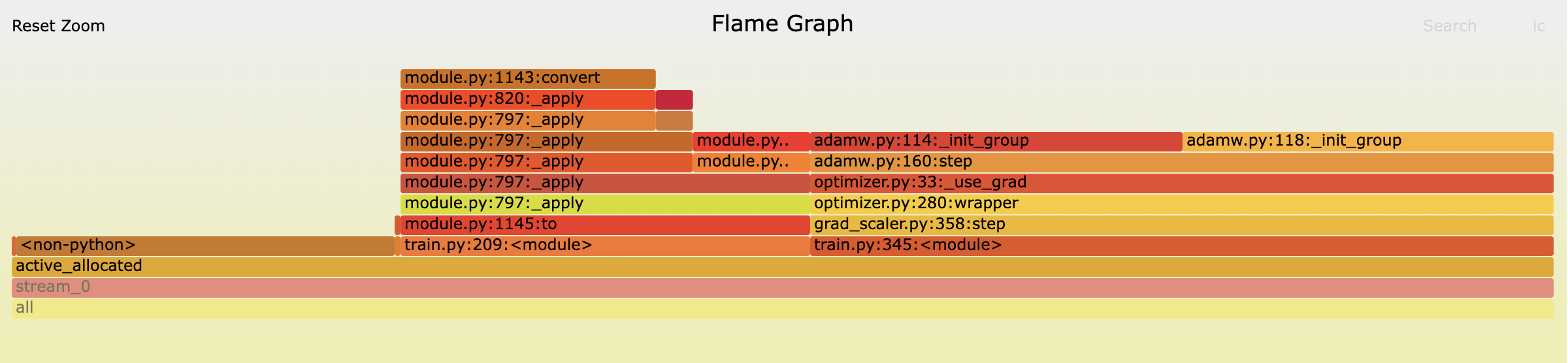
The table below shows a comparison to the bytes seen on the segment above and my predicted values. We come very close and the vast majority of the difference is accounted for by “gaps” which are caused by the allocated block size being larger than the tensor in that block (source) because of the rounding up of tensor sizes to block sizes in the caching allocator.
| GPT2 Small | Predicted | Actual | Diff |
|---|---|---|---|
| N Parameters | 124,373,760 | 124,373,760 | 0 |
| Model Memory (bytes) | 547,826,688 | 547,826,688 | 0 |
| Gradients (bytes) | 497,495,040 | 497,495,040 | 0 |
| Adam buffers (bytes)1 | 994,990,080 | 994,990,380 | 300 |
| CuBLAS workspace (bytes)2 | 17,039,360 | 17,039,360 | 0 |
| Gaps (bytes) | 6,855,368 | - | |
| Inputs / Targets (bytes) | 196,608 | Not visible | - |
| Others not visble on segment (bytes) | 196,620 | - | |
| Total (bytes)3 | 2,057,547,776 | 2,064,403,456 | 6,855,680 |
1 summing the bytes in `adamw.py:114._init_group` blocks in the snapshot does give us exact agreement so there are some other (small) tensors being allocated by the optimizer.
2 see CuBLAS workspace section below.
3 actual as reported by torch.cuda.memory_allocated()
Pulling together the formulas above we can calculate the steady state memory usage of a transformer model as:
\[M_{\text{steady_state}} = 16N_{\text{param}} + 4N_{\text{buf}}\]Peak memory usage
The more interesting question pertains to calculating the peak memory usage of the model during training. This will occur towards the beginning of the backwards pass when in addition to the tensors above we also have the cached activations of the model in memory.
I consider the contributions of the activations from the different model components in turn. Throughout the layers of the transformer we repeatedly manipulate tensors of shape $\mathbb{R}^{\text{Bsz} \times T \times D_{\text{model}}}$ so define $N_{e} = \text{Bsz} \times T \times D_{\text{model}}$ as the number of elements in this embedding tensor. This comes up a lot so I will use this notation throughout.
Layer norm
Layers norms are calculated in FP32, e.g. see list of autocast compatible ops here. So for each layer norm we need to store input activations of size $4N_{e}$ bytes.
Attention block activations
In the attention block of a transformer there are the following operations which contribute to the activations:
- Layer norm: Store $4N_{e}$ bytes
- Linear layer for calculating the $Q$, $K$ and $V$ matrices: Calculated as $[Q, K, V] = XW_1$ in half precision so need to store $X$ which is $2N_{e}$ bytes
- Matrix multiplication for $P=QK^T$: Store $Q$ and $K$ in half precision so $2 \times 2N_{e}$ bytes.
- $\text{Softmax}(P)$: Store $P \in \mathbb{R}^{\text{Bsz} \times N_{\text{heads}} \times T \times T}$ (let $N_{a} = \text{Bsz} \times N_{\text{heads}} \times T^2$), softmax is done in FP32 so $4N_{a}$ bytes
- Matrix multiplication for $S=PV$: Store $P$ and $V \in \mathbb{R}^{\text{Bsz} \times \text{seq} \times D_{\text{model}}}$ in half precision so $2N_{a} + 2N_{e}$ bytes
- Output linear layer $Y = SW_2$: Store $S \in \mathbb{R}^{\text{Bsz} \times T \times D_{\text{model}}}$ in half precision so $2N_{e}$ bytes
Total memory usage for the attention block is therefore:
\[\begin{align} M_{\text{attention}} &= 4N_{e} + 2N_{e} + 4N_{e} + 4N_{a} + (2N_{a} + 2N_{e}) + 2N_{e} \\ &= 14N_{e} + 6N_{a} \end{align}\]Feed forward block activations
In the feed forward block of a transformer there are the following operations:
- Layer norm: Store $4N_{e}$ bytes
- First linear layer $Y = XW_1$: Store $X$ so $2N_{e}$ bytes
- GELU: Store $Y$ so $8N_{e}$ bytes (as $W_1 \in \mathbb{R}^{D_{\text{model}} \times 4 D_{\text{model}}}$)
- Second linear layer $Z = AW_2$: Store $A$ so $8N_{e}$ bytes
Total memory usage for the feed forward block is therefore:
\[\begin{align} M_{\text{ff}} &= 4N_{e} + 2N_{e} + 8N_{e} + 8N_{e} \\ &= 22N_{e} \end{align}\]Other transformer operations
- Final layer norm: Store $4N_{e}$ bytes
- Head linear layer (to calculate logits): Store $2N_{e}$ bytes
There are also the activations associated with the initial embedding matrix and positional embeddings. However because the inputs to these are shaped $X \in \mathbb{R}^{\text{Bsz} \times T}$. These are very negligible compared to the other activations so I will ignore them.
\[M_{\text{other}} = 4N_{e} + 2N_{e} = 6N_{e}\]Cross entropy
For the cross entropy loss we need to store the logits. The logits are $L \in \mathbb{R}^{\text{Bsz} \times T \times D_{\text{vocab}}}$ (let $N_l = \text{Bsz} \times T \times D_{\text{vocab}}$). Additionally from inspecting the trace below (click for interactive version) as part of the forwards pass PyTorch is storing an FP16 copy of the logits and (I infer) an FP32 tensor of the same size as the logits. So the total memory usage for the cross entropy is $2N_l + 4N_l = 6N_l$ bytes (these correspond to the green and yellow blocks below, the purple block is allocated after .backwards() is called so I account for this later as it is technically not an activation).

First block labelled 'Logits (fp16)' are the logits returned by the model and the allocations labeled 'Stored' correspond to activations saved during the cross entropy loss calculation.
The combined formula for the memory usage of the activations in bytes is therefore:
\[M_{\text{activations}} = N_{\text{layers}} \times (36N_{e} + 6N_{a}) + 6N_{e} + 6N_l\]where
\[\begin{align} N_{e} &= \text{Bsz} \times T \times D_{\text{model}} \\ N_{a} &= \text{Bsz} \times N_{\text{heads}} \times T^2 \\ N_l &= \text{Bsz} \times T \times D_{\text{vocab}} \end{align}\]The python function shows the same calculation broken down on a granular level.
def get_activations_mem(d_model, n_layers, vocab_size, bsz, seq_len):
    layer_norm = bsz * seq_len * d_model * 4  # FP32

    embedding_elements = bsz * seq_len * d_model   # Number of elements (comes up a lot)

    # attn block
    QKV = embedding_elements * 2  # FP16
    QKT = 2 * embedding_elements * 2  # FP16
    softmax = bsz * n_heads * seq_len ** 2 * 4  # FP32
    PV = softmax / 2 + embedding_elements * 2  # FP16
    out_proj = embedding_elements * 2  # FP16
    attn_act = layer_norm + QKV + QKT + softmax + PV + out_proj

    # FF block
    ff1 = embedding_elements * 2  # FP16
    gelu = embedding_elements * 4 * 2  # FP16
    ff2 = embedding_elements * 4 * 2  # FP16
    ff_act = layer_norm + ff1 + gelu + ff2

    final_layer = embedding_elements * 2  # FP16
    model_acts = layer_norm + (attn_act + ff_act) * n_layers + final_layer

    # cross_entropy
    cross_entropy1 = bsz * seq_len * vocab_size * 2  # FP16
    cross_entropy2 = cross_entropy1 * 2  # FP32?
    ce = cross_entropy1 + cross_entropy2

    mem = model_acts + ce
    return mem
To check the accuracy of the activations calculations above lets take another snapshot after the forwards pass but before the backwards pass so we can see the activations in memory.
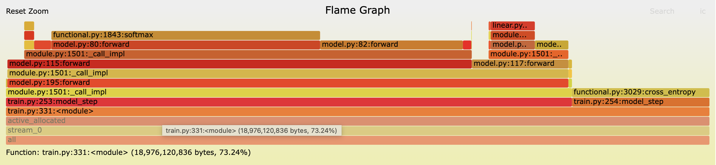
The snapshot shows 17.673GB of activations in memory. Using my function above I estimate 17.429GB which is pretty close again but there is c. 250MB of allocations unaccounted for by my estimate. From inspecting the traces and snapshots I notice that some of the linear layers are making some additional allocations that I am not accounting for. For example, the linear layers for the QKV matmuls are responsible for a total allocation of 256.5 MB (21.375MB per layer) whereas I only budget 18MB in my calculations above leaving a 3.375MB difference per layer. Some of the other linear layers show similar unexplained allocations. Whilst it pains me not to account for every byte I am going to ignore this for now and move on.
Comparing to EleutherAI’s formula:
\[M_{\text{activations}} = T \times \text{Bsz} \times D_{\text{model}} \times N_{\text{layers}}(34 + 5\frac{N_{\text{heads}}T}{D_{\text{model}}})\]we get an estimate of only 12.02GB showing the importance of taking into account the datatype that the activations are stored in.
Total peak memory
So we now have accurate estimates for the steady state memory usage and (slightly less accurate) estimates of activation allocations. We can now use these to estimate our peak allocated memory during training.
We saw from the trace in the cross entropy section that the peak memory usage occurs just after the start of the backwards pass when there is an additional allocation equal to an FP32 copy of the logits (purple block labeled “Start of backwards pass” in the trace). So to estimate our peak allocation we can just add this additional $4N_l$ bytes to our steady state memory usage and the activations.
Peak memory usage for a transformer is then given by:
\[\begin{align} M_{\text{peak_memory}} &= M_{\text{steady_state}} + M_{\text{activations}} + 4N_l \\ &= N_{\text{layers}} \times (36N_{e} + 6N_{a}) + 6N_{e} + 10N_l + 16N_{\text{param}} + 4N_{\text{buf}} \end{align}\]Using this formula we expect 21.648GB peak allocated memory for GPT2-small. pytorch.cuda.max_memory_allocated() returns 21.898GB and the 250MB delta is accounted for by the unexplained activation allocations mentioned above.
I plot a comparison of estimated to actual peak memory usage for various GPT2 models below I also include a line for the predicted steady state memory usage (i.e. exculding activations).

Comparison of estimated to actual peak memory usage for GPT2 small, medium and large.
Other considerations
This post has focussed on a rather vanilla implementation and there exist a number of tricks aimed at reducing memory footprint which I haven’t covered here. These include:
- Gradient checkpointing (save memory by recomputing some activations during the backwards pass)
- Tensor parallel (reduce the memory usage of the activations and weights by splitting the model across multiple gpus)
- Zero redundancy optimizer (reduce the memory usage of optimizer states by sharding these tensors across multiple gpus)
- FSDP (reduce the memory usage by sharding parameters, optimizer states, gradients activations across multiple gpus)
I may come back to cover these in a future post.
Thanks to Sam for reviewing an earlier draft of this post and providing some helpful feedback.
Appendix: some other uses of memory
CuBLAS workspace
One small (and interesting) use of persistent memory which is related to cuBLAS creating a workspace lazily on the first call to a GEMM. These pools are created thread locally (so we get one for the forwards pass and one for the backwards pass) and they use 8,519,680 bytes, e.g. sum the numbers on this line. Shout out to David Macleod for tracking down the sources of these allocations in the PyTorch source code!
The python code below demonstrates the appearance of these allocations:
def snap():
    return torch.cuda.memory_allocated()

print(f"Starting mem: {snap()}")
a = torch.randn(2, 2, requires_grad=True).cuda()
a.retain_grad()
print(f"Mem usage after allocating a: {snap()}")
out = a.mm(a)
print(f"Mem usage after matmul: {snap()}")
gradient = torch.randn(2, 2).cuda()
print(f"Mem usage allocating gradient: {snap()}")
out.backward(gradient)
print(f"Mem usage after backwards: {snap()}")

# prints:
Starting mem: 0
Mem usage after allocating a: 512
Mem usage after matmul: 8520704
Mem usage allocating gradient: 8521216
Mem usage after backwards: 17041408
We can see after the matmul there are an extra 8,519,680 bytes allocated (above the 512 bytes for the allocations of a and out). And an extra 8,519,680 bytes are allocated after the backwards pass (= 17,041,408 - 8,521,216 - 512) with the final 512 being the allocation of the a.grad that is created during the backwards pass.
Why 512 bytes? This is smallest block size that the caching allocator will allocate - link, so a tensor of size 512 bytes or less will result in an allocation of 512 bytes.
Cuda Context
Another large-ish source of memory usage is the cuda context. This is initialized as soon as your allocate your first a tensor to the gpu and takes up about 863MB. However this is not shown by torch.cuda.memory_allocated() or torch.cuda.memory_reserved(). But you will see it on nvidia-smi.
mem = snapshot_memory_usage()
print(f"Memory usage before generating data: {snap()}")
x = torch.empty(0).cuda()
print(f"Memory usage after generating data: {snap()}")
breakpoint()
Shows 0 bytes allocated before and after creating the empty tensor. But running nvidia-smi whilst on the breakpoint we see usage of 863MiB.
+-------------------------------+----------------------+----------------------+
|   2  NVIDIA A100-SXM...  On   | 00000000:43:00.0 Off |                   0* |
| N/A   32C    P0    71W / 400W |    863MiB / 81920MiB |      0%      Default |
|                               |                      |             Disabled |
+-------------------------------+----------------------+----------------------+